Spatio-temporal navigation

Warning: This documentation is out of date and does not describe the behavior of the latest major version 4, which implements a new model. An up-to-date documentation can be found in the program help.

Abstract

This first topic is intended to familiarize oneself with the simulator if one has not used it before. One objective is to show the basic spatial and temporal navigation functions. For this purpose, we will play around with an existing simulation file from the provided examples, which provides a (nearly) pure physics demonstration. In general, it is possible to equip cell clusters with functions that allow programmable interaction with the environment.

Open a simulation file

We open a prepared simulation file by clicking on Simulation in the menu and then on Open. When the corresponding dialog appears we navigate to the directory ./examples/simulations/physics and select ALIEN.sim. Generally, every ALIEN simulation consists of 3 separate files. In this case we have the following:

• ALIEN.sim - This is the main simulation file and the one which is shown in the dialog. It contains every particle that is in the simulated world. It should be noted here that sim-files can also be loaded in the pattern editor. But in that case no settings and symbols are changed.

• ALIEN.settings.json - All simulation settings including world size, time step, simulation parameters and zones are stored here. These include, among others, physical parameters responsible for damaging, bonding or radiation of bodies. All this properties are encoded here in the JSON format and can thus be edited outside with any editor.

• ALIEN.symbols.json - In this file one finds a list of symbols and their defining values. Symbols are user-defined simple substitution rules and are used to simplify the writing of small programs in a certain assembler-like language for computing cell functions. Symbols can be constants or variables.

Spatial navigation window

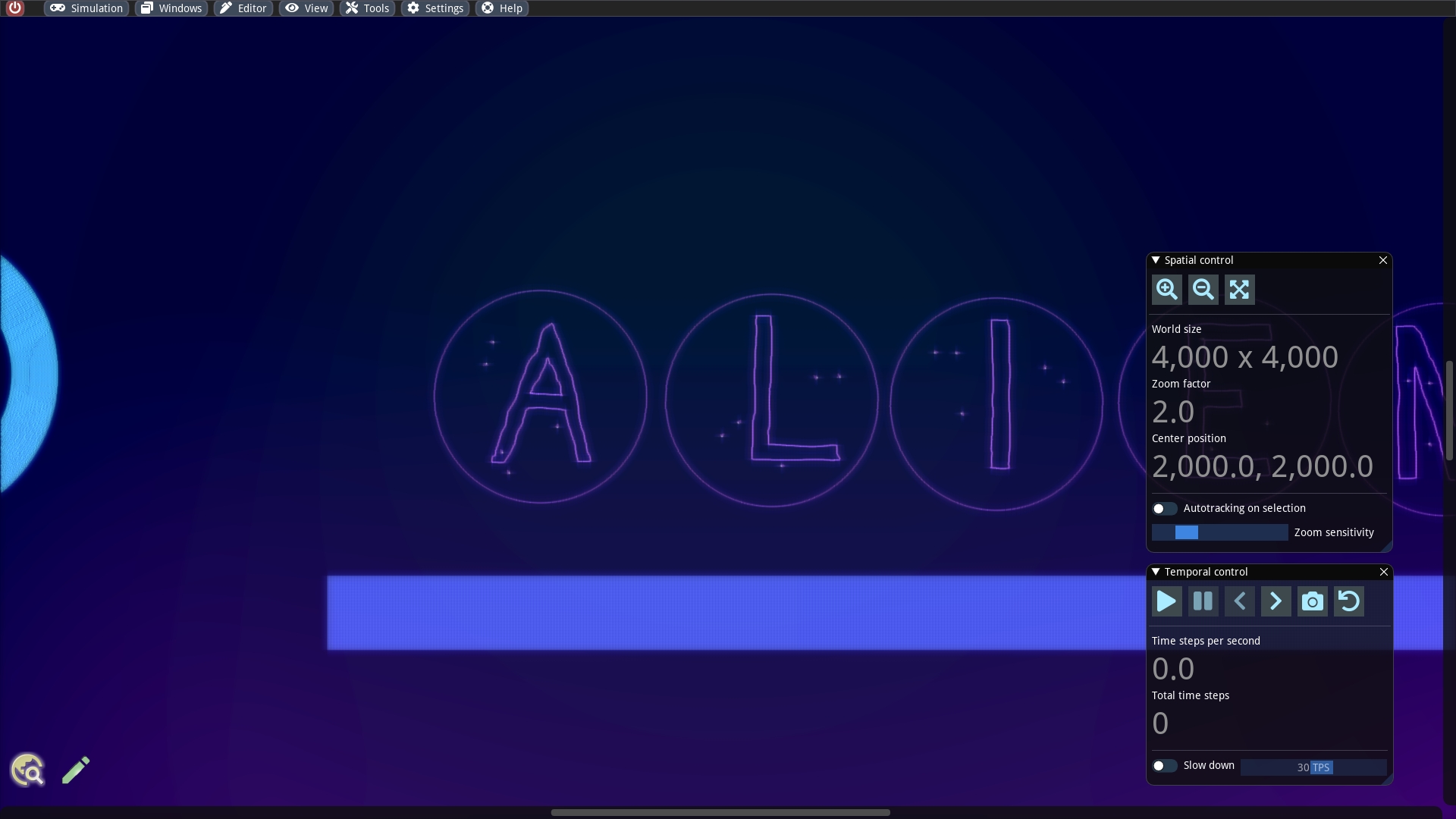
After opening the file, the view is centered, the zoom level is set to 2.0 and the simulation is paused. By default the two windows Spatial control and Temporal control are visible on the right. If not they can be activated in the Window menu. In this section, we are particularly interested in the spatial navigation window. You should see the following:

Initial configuration after loading ALIEN.sim

The purple color gradations in the background result from zones with different simulation parameters, but here they serve more as a visual decoration.

By default, the navigation mode is enabled (or in other words: the editor is deactivated). In this situation we can navigate with the mouse as follows:

• If we press and hold the left mouse button, we zoom in the direction of the mouse cursor.

• If we press and hold the right mouse button, we zoom out.

• If we press and hold the middle mouse button, we can scroll by moving the mouse.

The zoom speed can be adjusted with the slider next to the label Zoom sensitivity in the spatial control window.

For large worlds, navigation via the scroll bar on the right and at the bottom of the simulation view are also useful, as well as the zoom icons in the window.

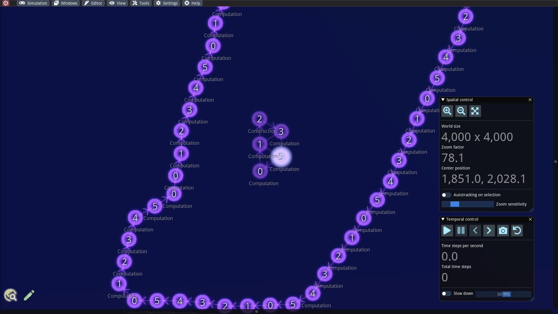
When zooming in, one notices that more and more additional details are faded in:

• At the coarsest level, the cells and particles are displayed only as small dots.

• From a zoom level of 4 and more, connections between the cells can also be recognized.

• If you zoom in even further, the token pathways can be identified by arrows. Optionally further information can be displayed by activating the Information overlay in the view menu. In this case also the cell specializations and token branch numbers are displayed as labels next to the cells.

High zoom level with information overlay

For the sake of completeness, it should be noted here that the world size can be adjusted in the Spatial control window. In addition, the view can be automatically centered on the selection (if there is one) when the simulation is running. For this purpose there is the toggle next to Autotracking on selection. We will discuss these functions in later tutorials.

Temporal navigation window

We can now start the simulation by clicking on the play icon in the Temporal control window. This window also shows the execution speed and the time steps calculated so far. Besides the play and pause icons, one finds the following useful functions:

• Move a single time step forward: This function can be reached via the > button.

• Move a single time step backward: This function can be reached via the < button. This only works if a single time step has been calculated beforehand.

• Make a snapshot: The entire world is stored in the memory. This function can be accessed via the camera button. Note that only one snapshot can be taken. Clicking the camera again will delete the previous snapshot.

• Restore the previous snapshot: After a snapshot is created, one can invoke the restore button. Then one finds the entire simulation in the state of the snapshot. This also works in a running simulation (... and is fun! Please try it.). A snapshot can be reused, or in other words, it will not be deleted after restoring.

For convenience, a snapshot is always created when loading a new simulation. This allows one to return to the initial state without having to reopen the simulation file.

A very useful feature is to limit the computation speed, which can be done via the Slow down toggle. With a particularly low speed, the individual particle movements and cell functions can be better observed.